Excel is probably the best known and used tool for general purpose management tasks. For that reason, when a project manager needs to create a Gantt chart for his project Excel is the first option.
Here, we explain to you how to create a Gantt chart in Excel step by step.
Create a project plan
Open Excel and enter your project plan data into a worksheet. Use columns to represent the different aspects of your plan, such as activity description, start date, end date and duration.

Add a bar chart
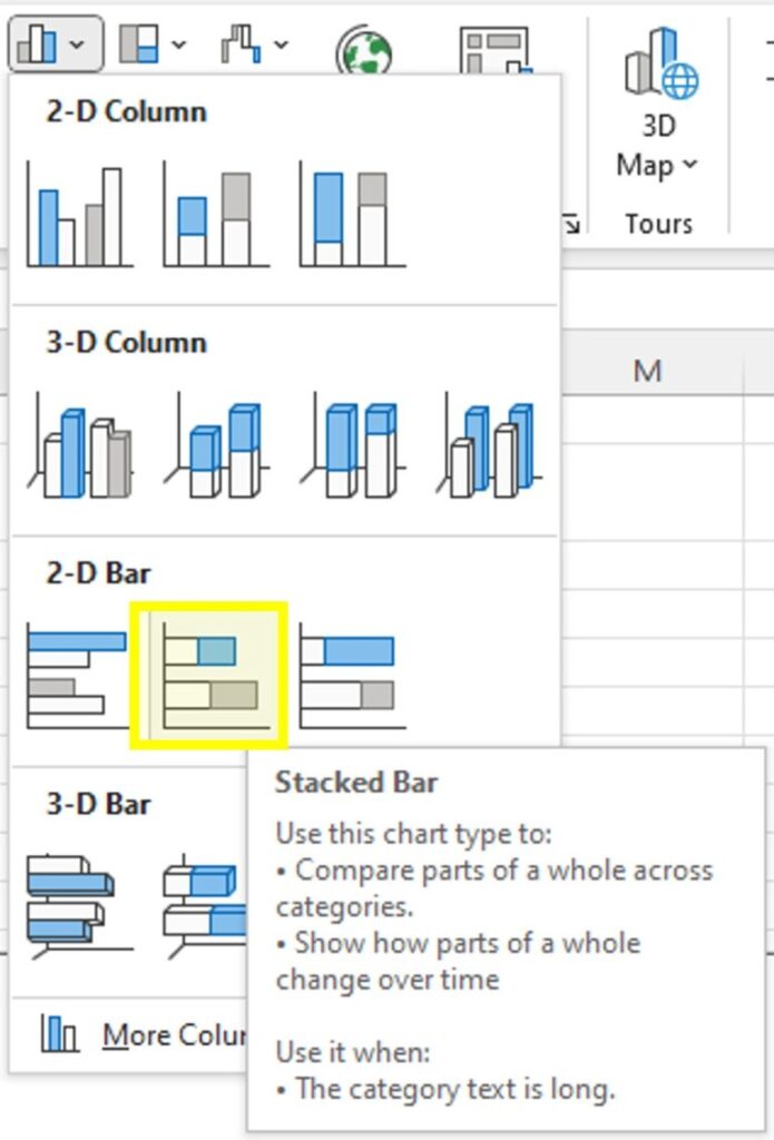
Click on the Insert tab at the top of the Excel window and select the “Bar” chart option. Choose the “Stacked Bar” chart type.
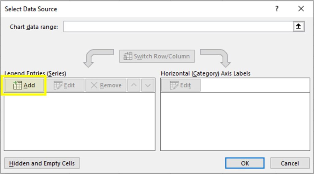
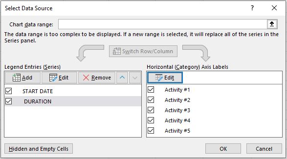
Now, right click on the bar chart area and click on Select Data. Click on Add to create two new data series.
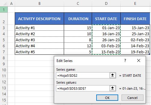
The first data series we need to select is the Start Date.
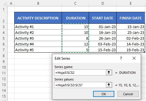
The second data series will be the Duration.
For the Horizontal Axis Lable we select the Activity Descriptions.
At this point, your chart should look something like this.
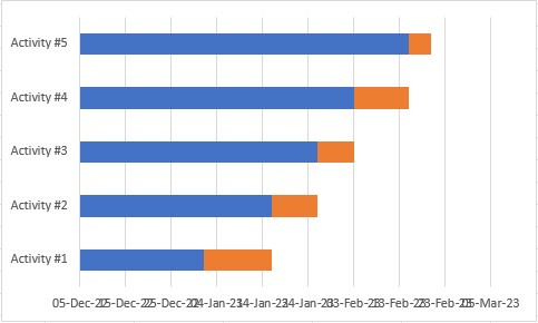
Format the chart
Once the chart appears, you can format it to look like a Gantt chart.
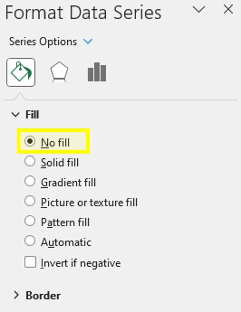
Let’s start by hidding the blue series of our stacked bars chart. Click on any of the blue bars (and check that the rest of the blue bars are automatically selected as well), right-click on the selected bar and click on Format Data Series.
A pane on the right will open. Select the Fill & Line section and change the Fill option to No fill.
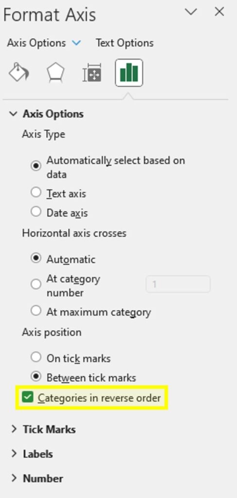
Next, we are formatting the Activities Axis. Since the format pane is already opened we only need to click on the Activities Axis to change the area we are going to format.
We want to reverse the order of the data series. Select the Axis Options and mark the check box for the Categories in reverse order option.
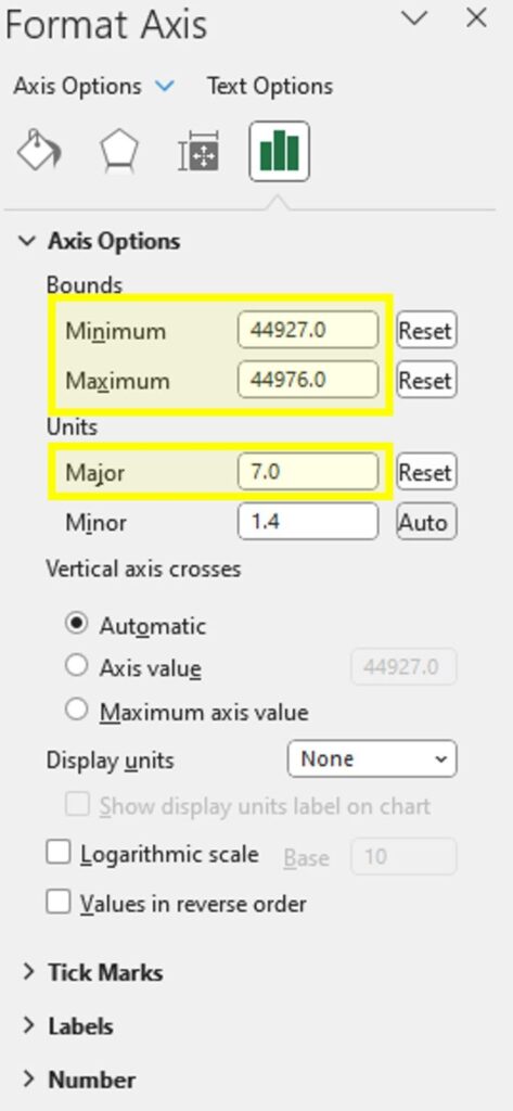
Finally, we are going to edit our Dates Axis. Click on the Dates Axis and select the Axis Options. Here, we are going to adjust the start and finish dates of our project and the period between shown dates.
To adjust the the start and finish dates of our project we need to introduce the start and finish dates in number format. To know the equivalent number to your start and finish dates select both in your activities table and in your ribbon click on Home>Number>Comma Style.
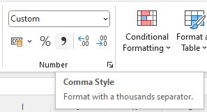
In this example, the project start date is the 01/Jan/2023, equivalent in number format to 44927, and the finish date is the 19/Feb/2023, equivalent in number format to 44976.
Besides, we want to show a date every seven days in our chart.
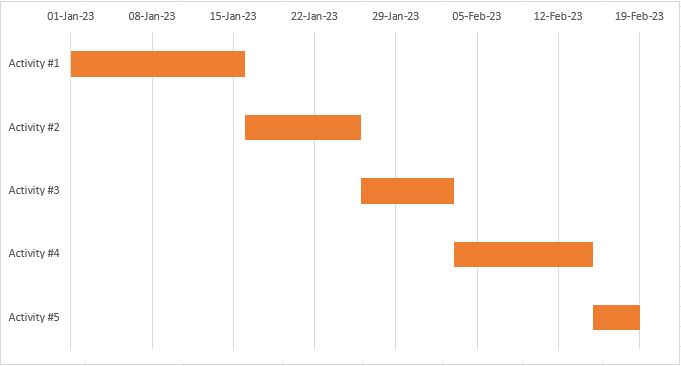
Your chart should look something like this.
Add additional formatting
You can further customize your Gantt chart by adding additional formatting, such as changing the chart and background colors or the axis font.
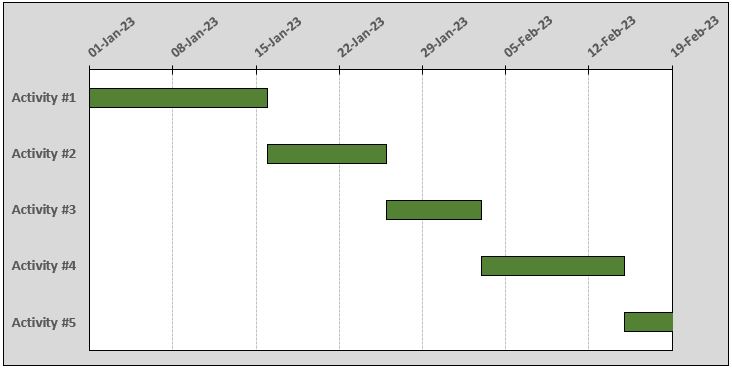
That’s it! With these steps, you can create a Gantt chart in Excel to help you visualize your project schedule and track progress over time.
However, this solution to create Gantt charts in Excel is less than perfect. Some of its drawbacks are that adding new activities is not agile or flexible, milestones cannot be represented and progress cannot be tracked.

